Hi everyone. The video on my YouTube channel has just over 1.5k views, which for a small channel is a decent accomplishment, but after a couple of recent emails, I realized that I had not linked to the ‘blank’ spreadsheet on my site, so here it is:
Now, as you may or may not know, I use LibreOffice Calc as my primary document creation, and this file is in .odt format. However, all the formulas use the Excel format, so you should be able to open this file in Excel, save it as an .xls or .xlsx file without issue.
When your taking a snapshot of the teams attributes every 3-4 months, and then the year to year comparisons, the number of tabs starts to add up. I think I am up to about 25, and while that’s still not anywhere close to the “Cry for help!” stage, it’s starting to be a concern…
Many of the pages continue to evolve, mostly due to suggestions from others. One very good suggestion comes from Ponzie on the Football Manager Slack channel, who asked if it wouldn’t be possible to get a table layout of a player progression, and then see how their attributes have improved over time. And with a little help from Google and Stack Exchange, it turns out there is.
For tracking a players improvement in another manner
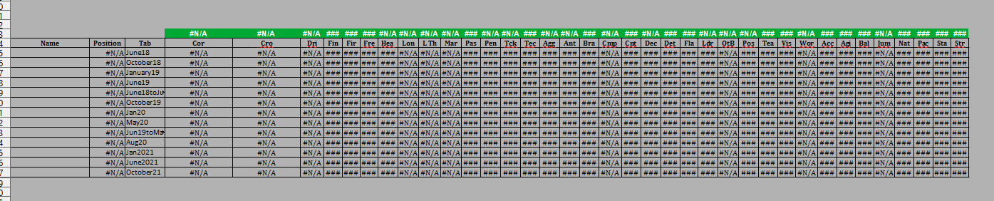
This is essentially the player attributes copied multiple times, with a column for the Tab being referenced. Now, I will be the first to admit I have no idea what exactly the formats used in the conditional formatting mean exactly, but here is what they are:
This formula gives a Red colored cell background if the condition is met.
Now, the VLOOKUPS used to populate the attributes are also there, what these two new formulas do is compare the numbers in each column to the number above it. If the number being compared is greater than the number above, it will turn Green. If it’s lower than the number above, it will turn red. No change, and the cell doesn’t change color.
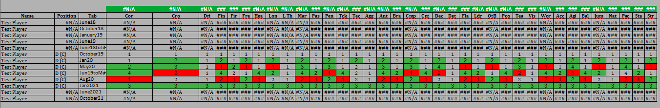
I created a player named “Test Player” on a couple of the previously built roster tabs. Here is what the results should look like when you get things typed in correctly:
Lots of pretty colors…
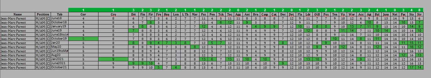
You’ll notice the number of color changes as the attributes improve or get worse. How does this look on a ‘real’ player? Well, lets take a look at one of the better youth players I have on my squad, Jean-Marc Parent. He’s been at Bastia since the beginning, and has turned into one of our best Midfielders.
Definitely has improved
Now, the row in Green across the top wit the white numbers is the total of ho much each category has improved. Some, like Strength, have improved quite a bit. Others, like heading, not so much. I use this to help me decide on training. In three years, his heading has improved by 1. That’s not so great, and leads me to believe that yes, while his Heading may improve over time, chances are slim it actually will, and the time spent practicing heading is probably better spent on First Touch, or Dribbling.
The nice thing about this section of the spreadsheet is that once the initial array in the formula is completed, you can insert as many lines as you would like, and the array will adjust to the new lines. I currently just have lines for most of the tabs I’ve already created, but as I continue on with the save, I can easily add more.
Now, these next couple of tabs I use could possibly be done a quicker, better way. I am open to suggestions on that, but for the moment, they take up the majority of the ‘behind the scenes’ work to get done.
First up: Wages.
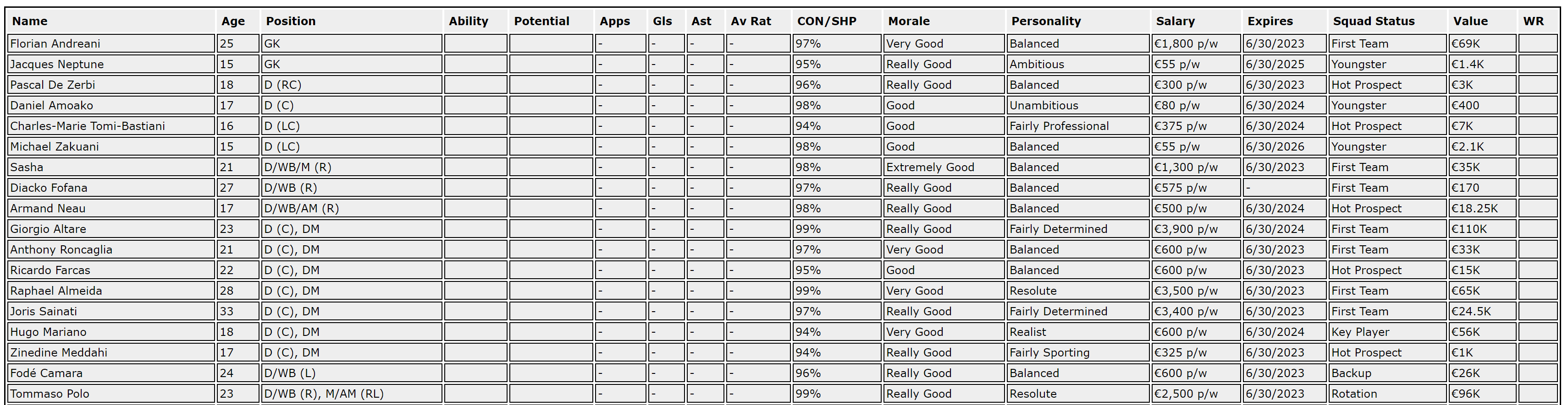
Now, the issue with this is the export from Football Manager. The format it uses, neither Excel or Calc really like, so you have to do some editing to make this:
Look like this:
I don’t want to get into all the nitty gritty behind the scenes stuff you have to do, but I will say that after the first couple of time you do the copy/paste, editing, and formatting, it goes by a lot quicker.
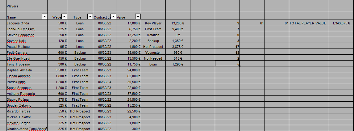
You’ll notice I’ve distilled the exported view down into the necessary columns for this, Player Name, their Wage, Contract Type, Contract End Date, and Value.
Next to that is another couple of columns, and using the formula:
=COUNTIF($D$4:$D$67, “=???”) where ??? equals Contract type in Column J, it counts the number of Key Player, First Team, and so on contracts I have on the squad at the time this view was exported. Column H totals up each players salary depending on contract type, with the formula:
=SUMIF($D$4:$D$99,”=???”,$C$4:$C$99) again where ??? equals Contract type in Column J
I also have a couple of checks on the total number of players, the first ’61’ counts the number of players in column B, the second 61 sums the total of column J, and for fun I also add in the total value of my players at the moment. Yes, at the moment this total is very, very sad.
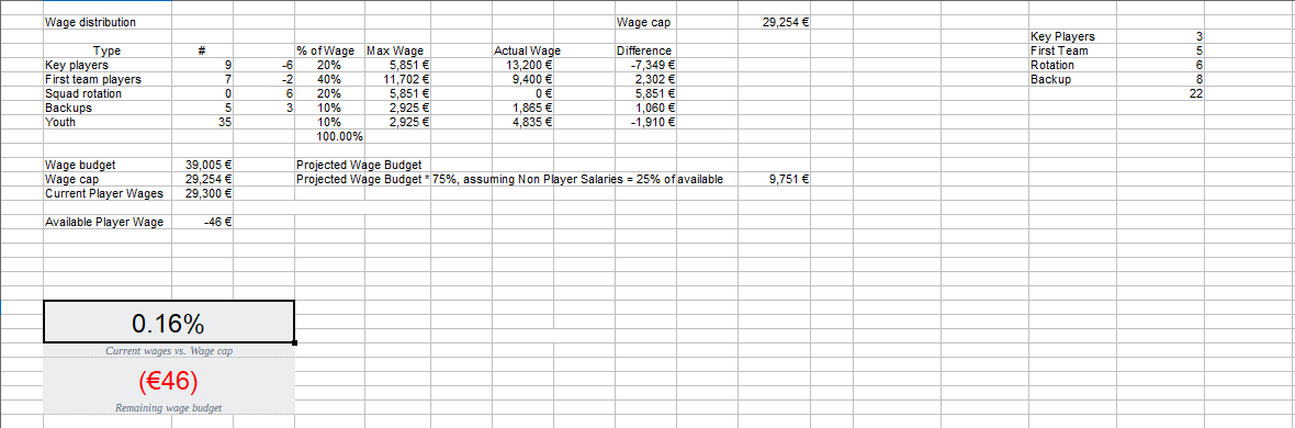
This tab then in turn feeds data to the Wage Distribution tab, which look like this:
It’s all nice and neat, of course it has to work…
The key number to look for here, and you know it’s key because it’s buried about halfway down, is the Wage Budget. This is the Budget the board set for me last season, €39,005. Now, the following is as best, a guesstimate with a dash of hunch and a smattering of “What could possibly go wrong here?” My assumption is that this year, my players salaries will account for 75% of my wage budget, meaning 25% of the wage budget is going to the coaches, scouts, physios and whatnot. I would think as you move up the leagues structure of whatever country you are in, and you get more Non Players as part of the club, this number could change some. I know when I started out in the National 3, I set it at 10%, because other than myself, a Chief Scout, and a Physio, we really didn’t have much else.
As you can see though, assuming 75% of our wage budget goes towards players salaries, we have a Wage Cap of €29,254.
The top part of this references data from the Players tab, with the Contract Type and number of contracts populated. You’ll notice over in column P and Q what I think a 22 man roster “should” look like, Column D is what I had at the time. I do not count Youth Contracts or hot Prospects as part of this. the ‘% of Wage’ Column is again, a guess. And then the number in Column F is what my max wage ‘should’ be, in this case three players on Key Contracts should be earning 20% of our entire wage budget, or €5,851.
I have 9 players earning €13,200….but I make up for that deficit by not having any Rotation contracts, and when all is said and done, you can see I am ‘ONLY’ €46 over my Wage Cap.
I find this useful especially when it comes to squad dynamics and playing time issues. If I have two (or more…) players on Key Contracts in the same position, you know the one that gets the least amount of playing time is going to complain about it sooner or later. Or, come the January transfer window, move some of the Key Players who aren’t playing so much out, and bring their replacements in on Squad Rotation contracts.
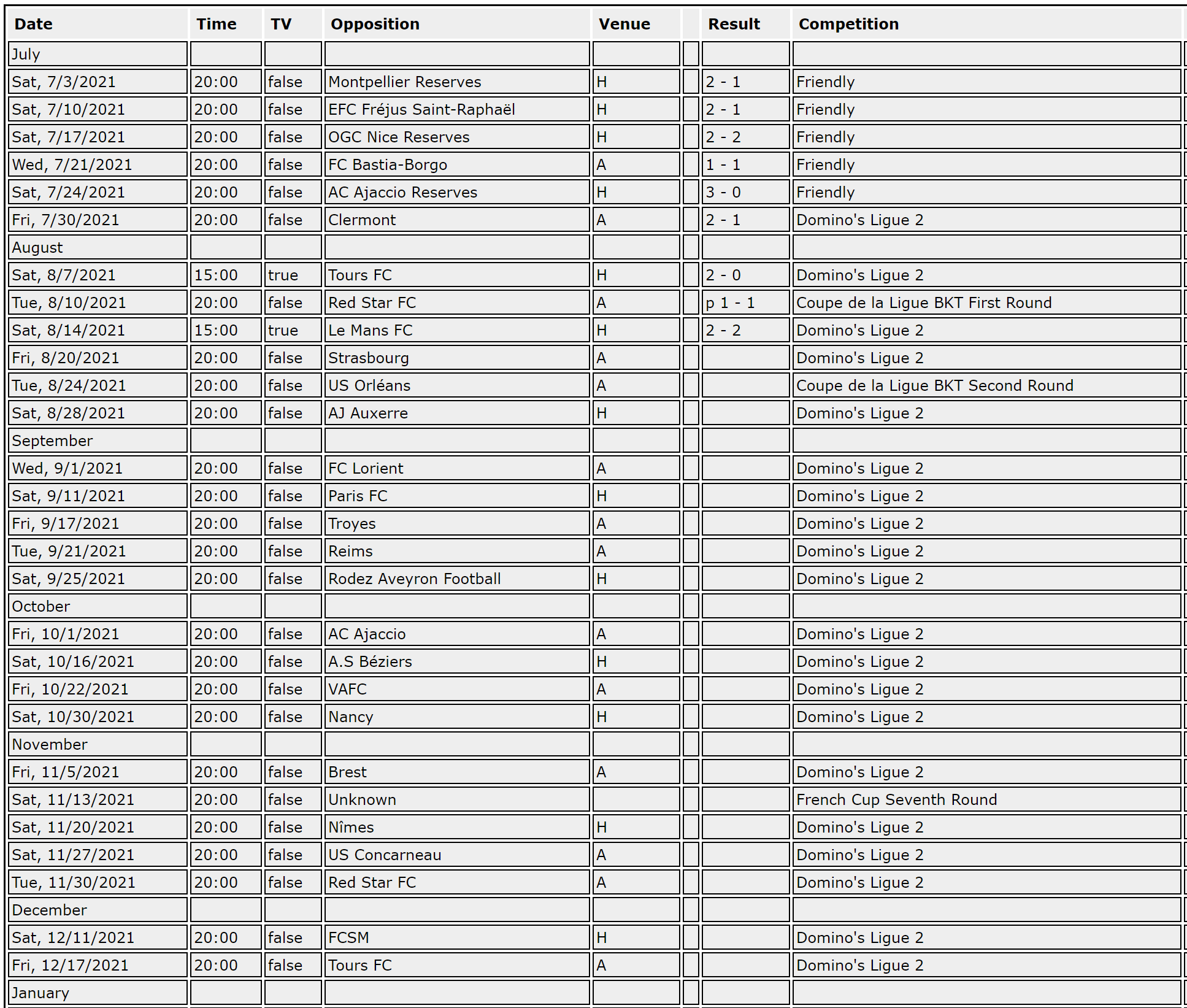
Last up for this post, the schedule. And I will admit, this takes a decent amount of behind the scenes work to get ready, and even then I still can’t make it do what I want it to do…yet.
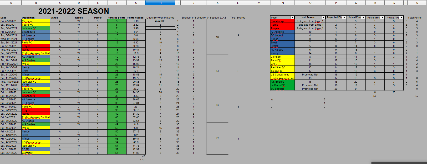
First, here’s what it looks like in all it’s glory:
It looks nice, but getting there can be a grind the first time
This was Bastia’s schedule in the 2021-2022 season. The video goes into a little more detail, and shows some of the changes when you switch a value, but for the moment, we’re going to start at Column N.
This is the teams in Ligue 2 at the beginning of the season.
Column O shows how they came to be in Ligue 2, and if applicable, where they finished the previous season.
Column P is the pundits prediction on where the teams would finish.
Column O is where they actually finished.
Columns R and S are the points Bastia earned Home and away at each opponent.
Column T is opponent strength, from 0 to 3. The teams in red get 3’s, blue gets a 2, Yellows 1, Greens 0. This represents how hard/easy I think it will be to beat them.
Starting in column A is the schedule, which I exported from FM with just the Ligue 2 fixtures on it.
Column J is the Strength of Schedule, change that number, and I have a conditional format that changes the background of the team cell.
Column D is the game result, type in W, L or D and Column E Populates.
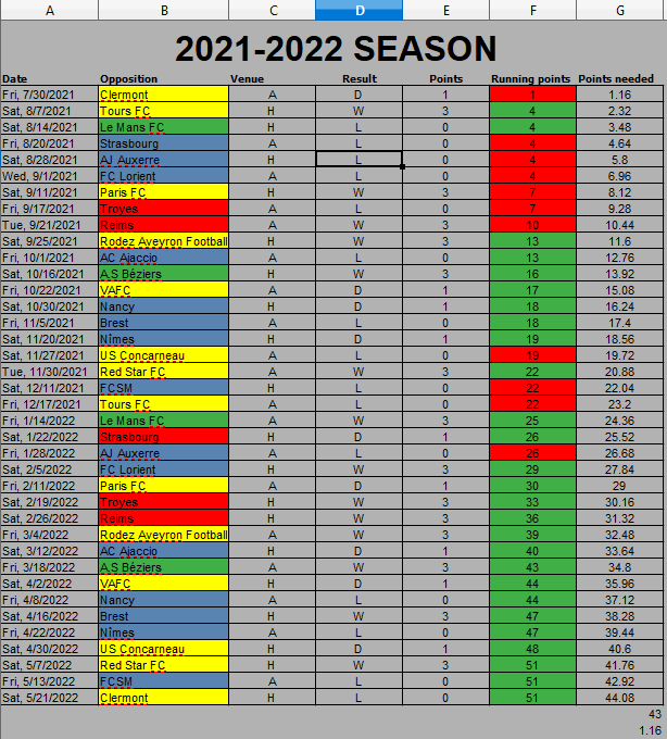
Column F is your running points total, and if more than the number in Column G, your running points total will be GREEN, if less it will be RED, like so:
If your in the red at the end of the season…
How did I arrive at Column G, Points needed? I went back and looked at the last 10 years of teams in Ligue 2, and found that you needed, on average, 43 points to avoid relegation. Add 1 to that you get 44 points. Divide 44 by 38 games played, you get 1.1578947…well, 1.16.
So, every game I played I needed 1.16 points to avoid relegation.
Column H counts the number of days between matches, but this isn;t the most useful at the moment, because this is just the basic Ligue 2 schedule. It does not include any Coupe de la Ligue, Coupe de France, or European Fixtures, because adding them in at the moment breaks some of the conditional formatting, and running points total. It’s something I am working on, but I will admit, I’m not working to hard on solving it at the moment.
Column I is Match Week number (Handy for when your sorting, and yes I learned this the hard way). Column J is the teams Strength of Schedule number, and the I break the league down into quarters, two of 9 games and two of 10 games.
What these tell me, and what the teams colors tell me, is what sort of battles I have coming up in the future, and how can I prepare for them better. You’ll see in the 1st Quarter of games I played five pretty good teams, but I want to highlight weeks 8, 9 and 10, when I played Troyes, Reims and Rodez Aveyron.
Troy and Reims are both quality teams, and I am playing them 4 days apart. 4 days after playing Reims, I am playing Rodez Aveyron, who are not that strong. Should I start my ‘A’ side against both Troy and Reims, and knowing they’ll be shattered from a condition point of view trust the Rodez game to my backups? What if this wasn’t the first quarter of the season, but the last, and I’m in a relegation battle? Whats sequence of games can I rest my started a little more, and play a more rotated side?
Now, the one downfall to this time at the moment I alluded to earlier: It doesn’t include non domestic league fixtures. IF/when I do get that figured out, it’s another tool to use in determine what the future looks like, and how to plan accordingly.
I can look at this all day long:
But for me, there’s not a lot of useful information there beyond the basics. And being a pretty visual person, doing what I do to the Schedule helps me plan more.
It shows some of the changes that happen when you change some of the values, and does go into a little more detail on the schedule side of things.
As always, if you have any questions or comments, leave them down below, or I can also be found at @FM_Jellico on Twitter. I also frequent the Football Manager Slack channels, and can also be found on the AbsoluteFM Discord server (amongst other Football Manager related Discords 🙂 )
And thats Part 2 of this series. Next up, in a couple of weeks, my Lineup Tab, also known as “How much Data can you have on one tab Jellico? JFC….”
I’ll be the first to admit, I am not the most knowledgeable soccer/football fan. I played it as a kid, followed it, although not too closely, when I lived in Europe in the 80’s, and while I know of the Premier League, Bundesliga and the like, until about 2017, my knowledge of world football was, at best, a PowerPoint slide or two deep. As an American, soccer/football just wasn’t something I followed too closely.
I am a gamer though. Board, miniatures, computer, pen and paper, dice, that was (and still is) a hobby of mine. There’s a Youtuber I follow named Quill18, who does a lot of “Let’s Plays” for various games I also play, and one day his followers challenged him to play FM17. And he did. And I sat there the whole time watching him play with a quizzical look of “What the hell is this and where has it been my life?” I know Madden, I like Madden and other sports games (Heck I was a Tecmo Bowl League my sophomore year of college, and yes, that makes me old), never played FIFA (because, well, Soccer…), but Football Manager was more than either of them. So, so much more.
So I bought it, and started to learn it. And two and a half years later, a couple of thousand watched videos on YouTube, and countless hours of streams by other content creators, it has become the game I play most. Like many games, it’s very customizable in the detail level you want, how much control you’d like. For most FM17, and most of FM18, I was a hands off coach. Tactics, some scouting, and press conferences, that was it. I spent a decent amount of time following up the scouts recommendations, but I never too full control of the club I was running.
That’s changed with FM19. After my initial Beta Test save (with Crystal Palace), I knew what save I wanted to do, and I also knew I wanted to exercise more control over, well, everything. But I needed some help to get that done.
In my day job, I’m a Geographer/GIS Analyst. I take data and represent it visually. Lot’s, and lots of data, and shapes, and details. I do also get to make some cools maps (Aswijan for example), but really, 75% to 90% of my job is manipulating data and making it not only understandable to the end user, but accurate as well. There’s a lot going on behind the scenes, and the end user will only see the last 10% or so of your efforts, but it’s the other 90% that makes things go.
On top of this, I am what I like to refer to as a “Least Amount of Effort” type of person. While that sounds bad, in actuality what it means is that if given a task, I’m not going to take any shortcuts to finish it, and I’m not going to add any chrome to it to make it flashier. If a job requires ten steps to get done, I’m going to do it ten steps. Not six, not fifteen, but ten.
I’ve been on projects with those sorts of people who do both. I’m not a fan.
I work with a lot of tables, and spreadsheets, and I like to be my job as easy as possible, so I will manipulate them to try and make my life easier. When it works, it’s great. When it doesn’t, well, thank god for CTRL-Z.
Early on, one of the things I wanted to do in FM17 with my first main save, was track how my players attributes improved. One of the things Football Manager is good at is the data it creates for, well, most everything. One of the things it’s not so great at is representing that data usefully. While that is a criticism, I understand why SI have done the things they have done when it comes to data and how they present it. But they do make it easy to export a lot of data, and with a little application of application, there are some things a manager can do to make his job a little easier. And that what I set out to do.
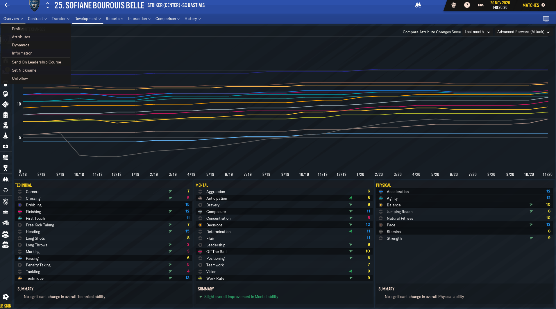
This is Sophiane Bouris Belle. He’s my very good youth striker in my current save with SC Bastia:
There’s a lot of data here, and a lot of it is quite useable. Attributed wise, I can tell by the little green arrows next to most of them that he is improving in all those areas. How much? Well, that’s where I run into some issues.
Clicking on Development→Attribute Changes gives you this screen:
Not a bad way to display this IMO, but there could be better ways.
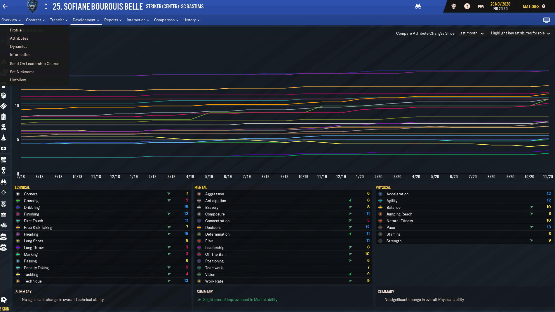
And it’s not bad, just incomplete, at least for what I want to do. Especially when you consider that if you turn on all the Attributes you get this:
To much data on one screen makes it unusable.
On some players, if you relax one eye you can see the sailboat…
But there’s better way of seeing these changes, at least for me.
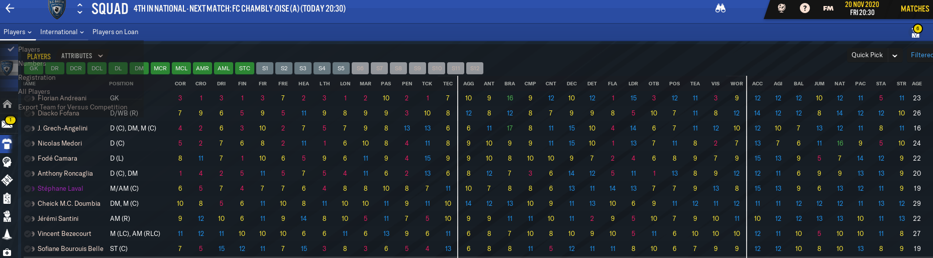
First, you have to create a Squad View of all the Attributes. And make sure the column order of this view is the same order as the player attributes. And do not mess with the columns after creating this view, or you will make a mistake. Yes, that’s from experience. You can add other items of info you want to the end, I find that makes it easier, but YMMV.
I Can’t stress this enough, don’t move these columns after you export the first time…
Now, open your spreadsheet program. I use Calc by Libreoffice, but I have it set up to use Excel formulas, so what follows should work without a problem on Excel.
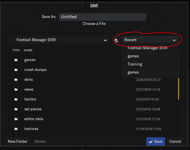
Now, go back into Football Manager, and under the FM button, scroll down to ‘Print Screen’ and Print as a Web Page, Select the folder you want to save it to, rename the file, to whatever you want, and click ‘Save’.
Helpful hint, if you have a set folder where you want all this data to go to, the next time you get to this screen, hit the ‘Recent’ drop down on the right, and a list of folders you’ve recently used, including the one your exported data is going into, should pop up.
A handy shortcut
Navigate to that folder, click the file, and it will open in your browser.
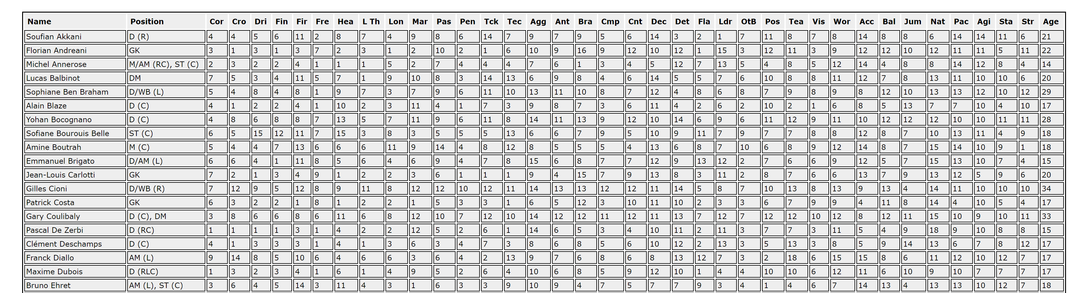
Basic HTML output.
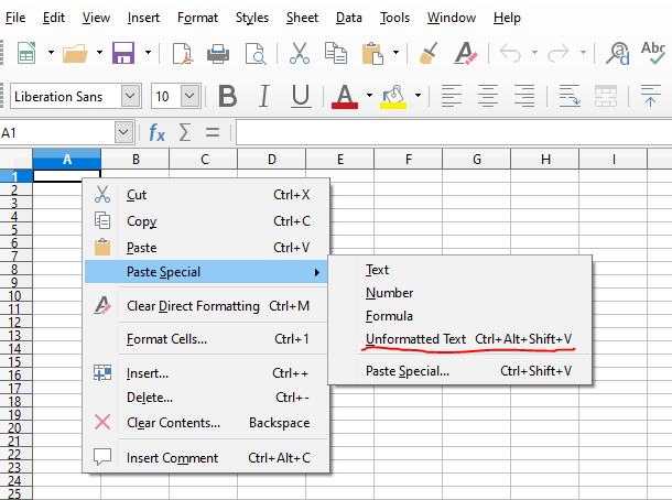
Select the data you want, copy it, go to your blank spreadsheet, select the cell you want the data to start in, and then this is very, very important:
Right Click, select Paste Special, and then select ‘Unformatted Text’
Very, very important!
This is very important, if you do not do this some formulas and calculations will not work!
This has to do with how Excel/Calc ‘see’s’ and interprets whats in the cell. Sometimes it sees ‘12345’ as a number, sometimes it sees it as text. Sometimes it will not ‘see’ text in a cell as part of a calculation, this is due to the cells format. Pasting everything in as ‘Unformatted Text’ should default most text to text, and numbers to numbers. There may be cases where you will have to go into the spreadsheet and set a cells format, but most of those occur later.
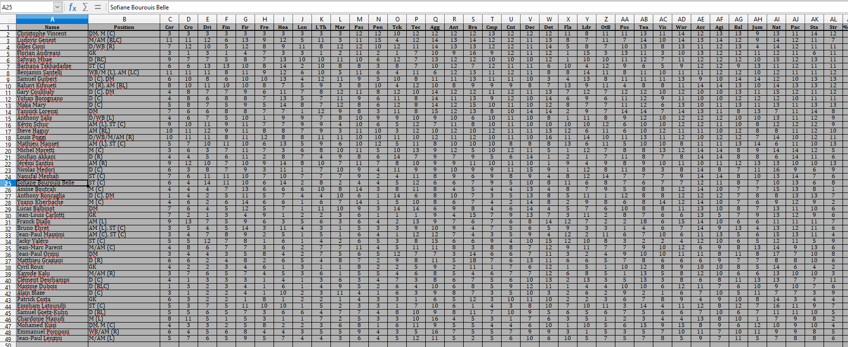
When you paste, you’ll get this:
And you can format this however you want. You will also want to rename the tab. I rename it whatever month I took the Attribute Screen Shot.
The next time you export an Attribute Screen Shot, create a second tab, cut and past the data the same way, and rename the tab.
NOTE: Your Attribute Screenshot does not have to have the names in the same order each time you take it. I promise.
Now comes the cool stuff: Conditional Formatting.
A conditional format is a rule you set up for data on the page, and that rule says that if a cell, or group of cells, is equal to the condition you set, whatever change you want to apply to that data will be applied.
Changes can range from font changes, to color changes, to both. You can have multiple conditional formats on a page, but you have to be careful how you apply them, as there is a priority/hierarchy to how they are applied.
Create a conditional format, set the condition to Formula Is and enter in the following formula:
C3<(VLOOKUP($A3,TAB!$A$2:$AL$99,COLUMN(),0)-1)
What I set for the style is to change the cell color to Red.
Now, an explanation of this formula, and what yoy may have to change to get it to work on your spreadsheet:
C3 is the first cell you want the formula to start looking at. Don’t use C2 if it’s your first line of data, the formula doesn’t like it. I’m not sure why.
A3 is the cell your Players Name is in.
TAB! is the name of the tab you want searched.
A$2:$AL$99 is the range of data being searched on the tab. This also means it will search all the data and names, including the first row.
So what this formula is saying is this:
Look at Cell C3. Compare it Value to the Value of the Cell where the name of the player in A3 of whatever tab your referencing; if that name isn’t in A3 search for it A2 to AL99, and once found, compare the numbers in the columns between the two tabs. If the number in tab2 is less than the number in tab1 by -2 (or more), turn the cell red. Clear as mud, right? I’m not sure how I could explain it better, any suggestions would be great!
The next formula should be:
C3>(VLOOKUP($A3,TAB!$A$2:$AL$99,COLUMN(),0)+1)
I set this to turn the cell dark green. This is looking for Values that are +2 or more that have changed between tabs.
Next formula is:
C3<(VLOOKUP($A3,TAB!$A$2:$AL$99,COLUMN(),0))
This is looking for Values that are -1 from Tab2 to Tab1, I set this to change the background to Yellow.
The last formula is
C3>(VLOOKUP($A3,TAB!$A$2:$AL$99,COLUMN(),0))
This is looking for Values that are +1 from Tab2 to Tab1, I set this to change the background to a lighter Green.
These formulas have to be entered in this order, when you arrange them in the condition box it has to read +2, -2, +1, -1.
This is because Excel and Calc are very hierarchy oriented, so if you have the -1 rule at the top, when the formatting formula is looking, it will see 8 is at least 1 less than 10, and turn it yellow, and because a condition has already been applied, it will not turn it read when it goes to apply the -2 change.
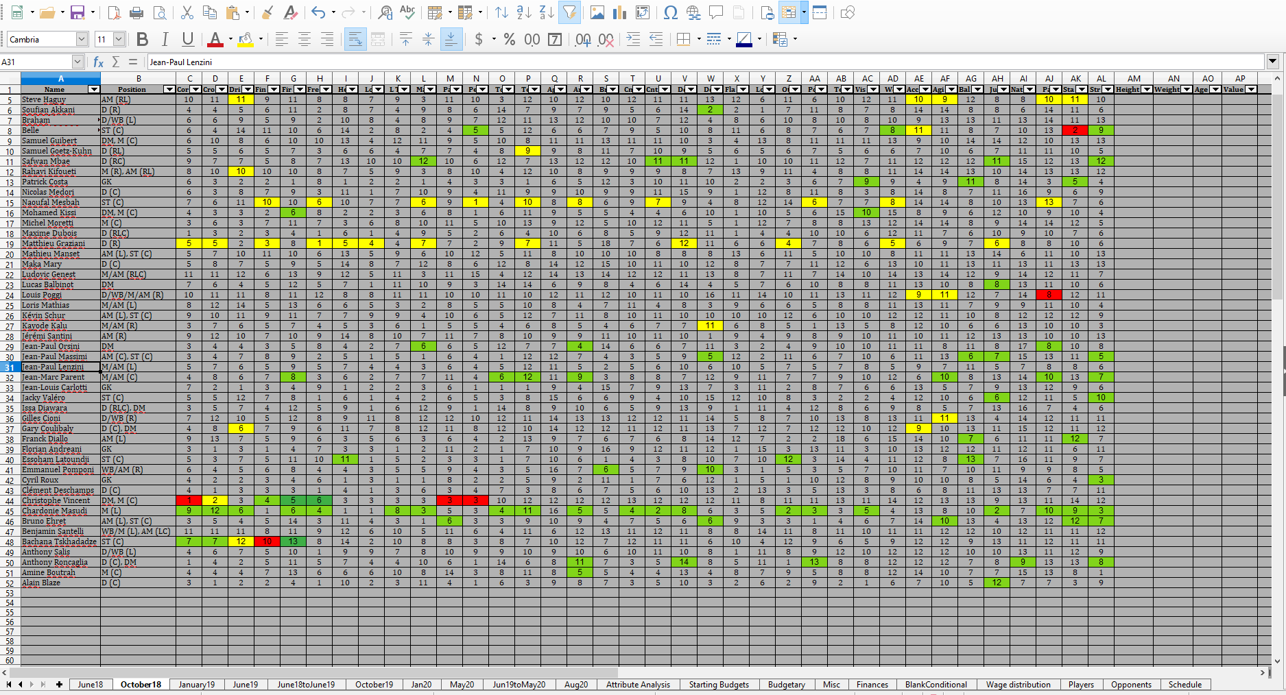
Once you have the formulas entered, hit ok/apply, they should take effect, and this:
I turn the background grey to cut down on glare. If you see my YT vids you know why.
Should turn into something like this:
Now how much easier is this to read?
When you need additional tabs, what I do is right click on an already filled out tab with the conditional formatting applied, copy it with a new name to the spreadsheet, then delete the names and data on the page. That way the formatting stays behind. The only thing you have to do now is go into the conditional formatting formulas and change the tab you want referenced.
One last note, which I mentioned before:
DO NOT MOVE ANY COLUMNS AROUND BETWEEN SCREEN SHOTS!
The formula used does not look at the column headers, but the Player Name, and once it finds the match, it will start comparing the values of the columns associated with that name from left to right. If you move the columns around between screenshots and apply the formula, you will get some strange results. I once couldn’t figure out how all on my players Physicals dropped -2, then found out I had deleted a column…
And that’s also the very cool thing about this formula, it looks at the name before it starts comparing. No matter where it is in the name column, if in your tab2 it finds the name in tab1, it will compare the numbers and apply the formatting.
As proof of this, the above is taken with the names in Ascending order.
This is a screenshot of the same tab with the names I descending order:
You’ll notice the formatting has moved with the player.
🙂
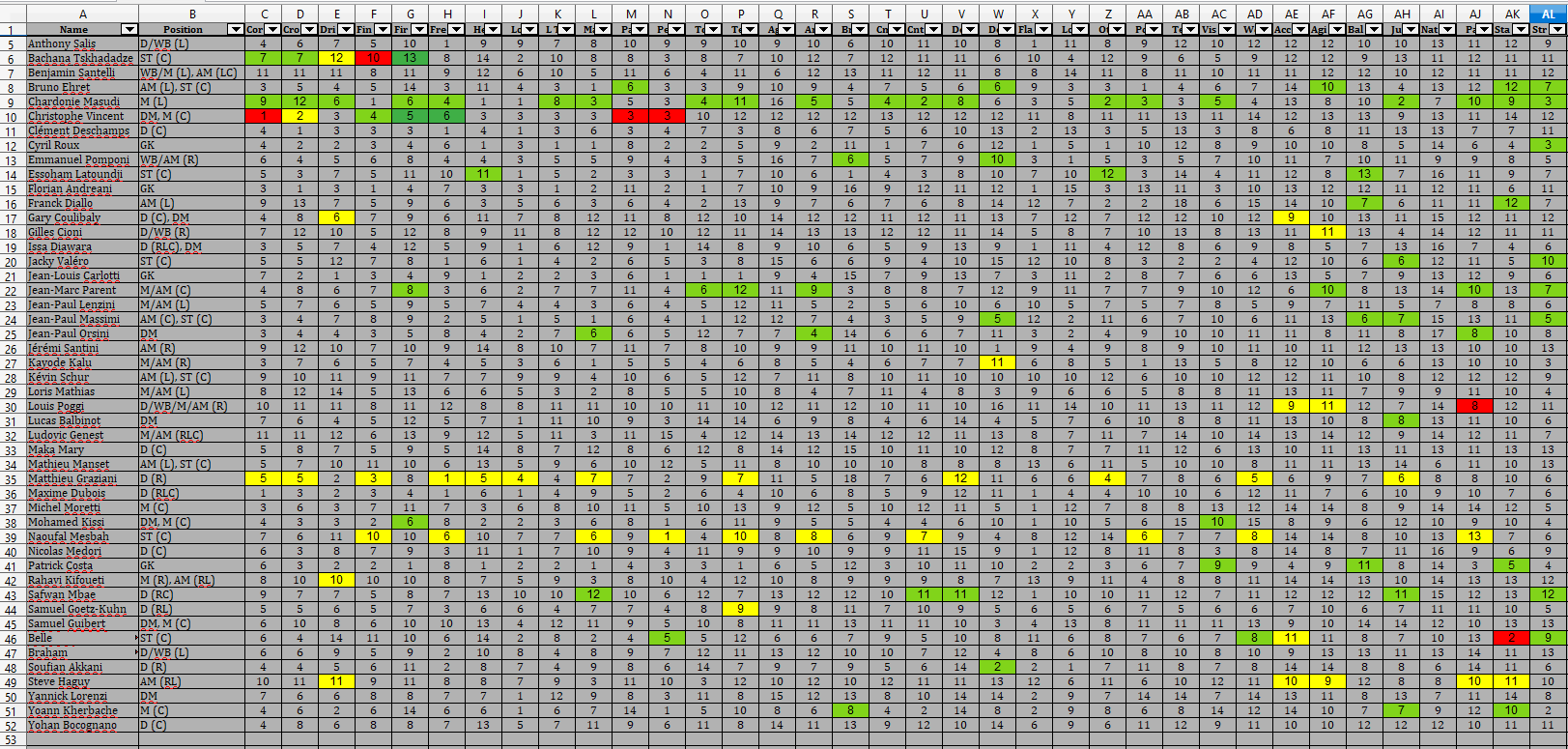
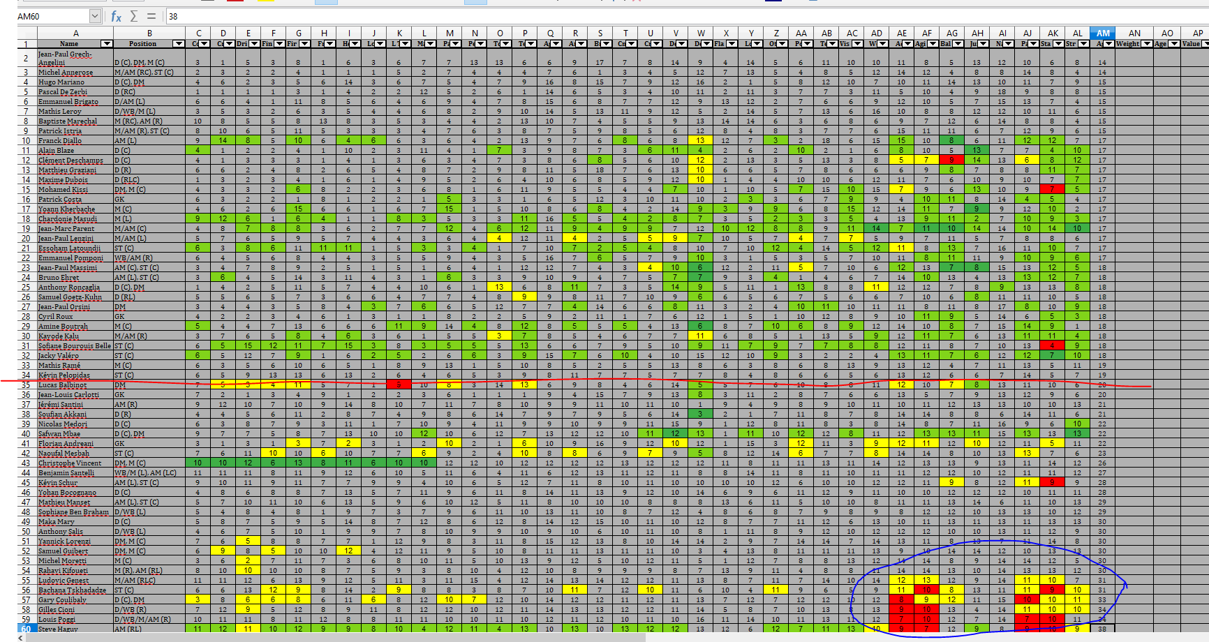
I’ve found this very useful for tracking not only my players growth every three or so months, but it’s also coming in quite handy as a training session aid as well. If my players are improving quite a bit in say their technical skills, but not their physical skills, I know I should start emphasizing more physically oriented training sessions. Likewise, it will show my youth players development, and when my older players start declining. This is a screenshot of my squad, comparing their progress from June of 2018 to June of 2019.
That’s a lot of green….
Everybody above the red line is a youth player.
The stats circled in blue are the physicals of my players aged 31 and older.
A little bit easier to interpret than a bar graph, right?
And that’s going to be it for Part 1 of this series. I don’t know how long it’s going to be to be honest, but I do know the next couple of parts are going to be the Attribute Analysis comparison graph, the Wage Budget Calculator I use, and the Schedule Tab, and all the things you can do with it.
A big thanks to the people over at the MrExcel forums (MrExcel.com) for help with a lot of the formulas used in this project.
Thanks for reading, and if there’s something you’d like to see please let me know.